Example of modelling: TOI-270

from pathlib import Path

import matplotlib.pyplot as plt
import numpy as np
import pandas as pd

plt.rcParams["figure.figsize"] = (10,5)

Matplotlib is building the font cache; this may take a moment.

To define a star:

from ravest.model import Star

star = Star(name="TOI-270", mass=0.386)
print(star)

Star 'TOI-270', 0 planets: []

Let’s define some planets. These parameter values for TOI-270 b, c, and d were obtained from Van Eylen et al. 2021. The full list of parameterisations supported can be seen at ravest.param.ALLOWED_PARAMETERISATONS.

from ravest.model import Planet
from ravest.param import ALLOWED_PARAMETERISATIONS, Parameterisation

print("Allowed parameterisations:", ALLOWED_PARAMETERISATIONS)

Allowed parameterisations: ['P K e w Tp', 'P K e w Tc', 'P K ecosw esinw Tp', 'P K ecosw esinw Tc', 'P K secosw sesinw Tp', 'P K secosw sesinw Tc']

parameterisation = Parameterisation("P K e w Tc")

planet_b = Planet(letter="b", parameterisation=parameterisation, params={"P": 3.3601538, "K": 1.27, "e": 0.034, "w": 0.0,   "Tc": 2458387.09505})
planet_c = Planet("c", parameterisation, {"P": 5.6605731, "K": 4.16, "e": 0.027, "w": 0.2, "Tc": 2458389.50285})
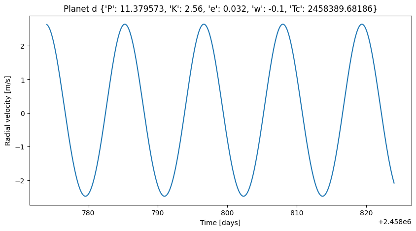
planet_d = Planet("d", parameterisation, {"P": 11.379573, "K": 2.56, "e": 0.032, "w":-0.1, "Tc": 2458389.68186})

We can see what the radial velocity would be due to the effect of one of the individual planets:

times = np.linspace(2458774, 2458824, 1000)

plt.figure()
plt.title(planet_d)
plt.xlabel("Time [days]")
plt.ylabel("Radial velocity [m/s]")
plt.plot(times, planet_d.radial_velocity(times))

[<matplotlib.lines.Line2D at 0x77d72f66a5d0>]

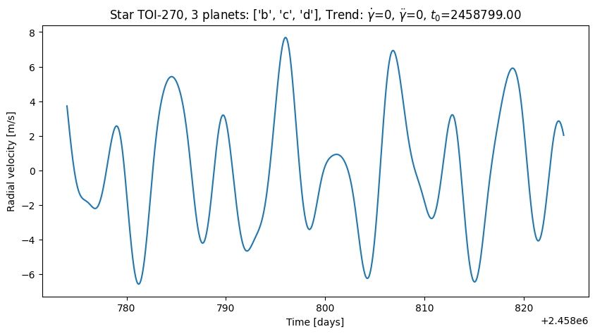
Let’s add the planets to the star, and use that to model the combined radial velocity that we would see, due to the effect of all of the planets. Notice that we also define a Trend object. This can store a constant velocity offset \(\gamma\) (\(\rm{ms}^{-1}\)), a linear trend \(\dot{\gamma}\) (\(\rm{ms}^{-1}/\rm{day}\)), and a quadratic trend \(\ddot{\gamma}\) (\(\rm{ms}^{-1}/\rm{day}^2)\), which are often used to account for e.g. instrumental contributions or possible undetected long-period companions. Trend also requires a reference/zero-point time \(t_0\) for the linear \(\dot\gamma(t-t_0)\) and quadratic \(\ddot\gamma(t-t_0)^2\) trend rates to be calculated from. I recommend to use the mean or median of the input times as \(t_0\).

from ravest.model import Trend

star.add_planet(planet_b)
star.add_planet(planet_c)
star.add_planet(planet_d)

star.add_trend(Trend(params={"g":0, "gd":0, "gdd":0}, t0=np.mean(times)))

plt.figure()
plt.title(star)
plt.xlabel("Time [days]")
plt.ylabel("Radial velocity [m/s]")
plt.plot(times, star.radial_velocity(times));

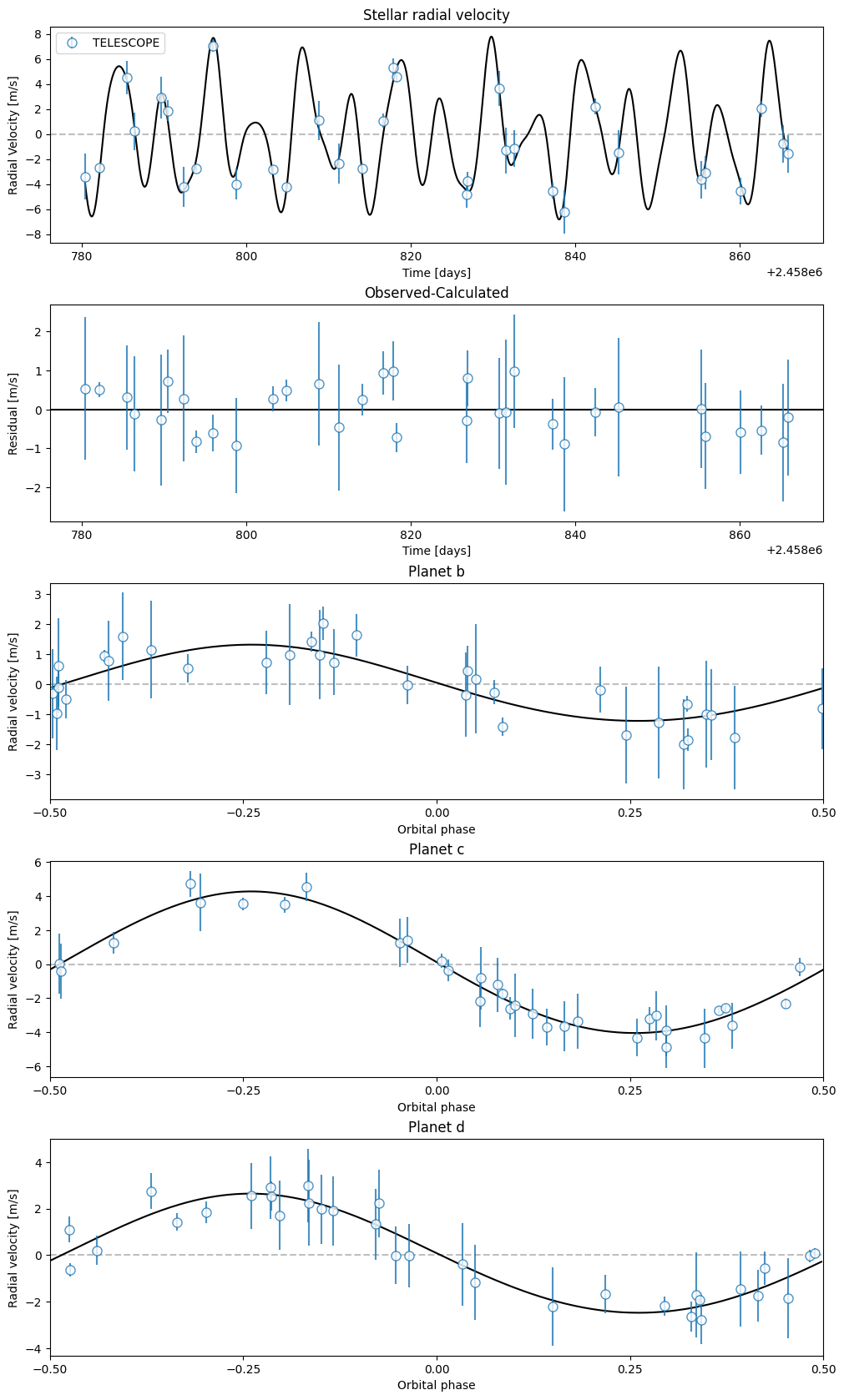
If we had some observed data, we can plot the data on top of the system RV model, and look at the residuals and generate phase plots for each planet. As a quick demonstration, I’ve previously generated some fake data for the TOI-270 system, which we can load in and compare our model to.

fpath = Path.cwd() / "example_data" / "TOI-270.csv"
df = pd.read_csv(fpath)
ti = df["ti"].to_numpy()
rv = df["rv"].to_numpy()
err = df["err"].to_numpy()
tel = df["tel"].to_numpy()
star.phase_plot(ti, rv, err, tel)

If you had some real data and you wanted to fit a planetary model to it, check out the tutorial notebook on fitting.